Quick start
VisualPDE is a web-based set of tools for solving partial differential equations (PDEs) via an interactive, easy-to-use simulation. To get started, try playing with some of the linear examples, or read on for some quick tips for using the solver.
Interacting with the simulation
Clicking/pressing on the simulation draws values right onto the domain. You can customise exactly what this does under → Brush For example, the default settings in the heat equation example allow you to paint ‘heat’ of value 1 onto the domain, which acts like an initial condition for the rest of the simulation. If you have another mouse button to press, you can use it to remove ‘heat’.
The equations panel
Pressing opens up the equations panel.
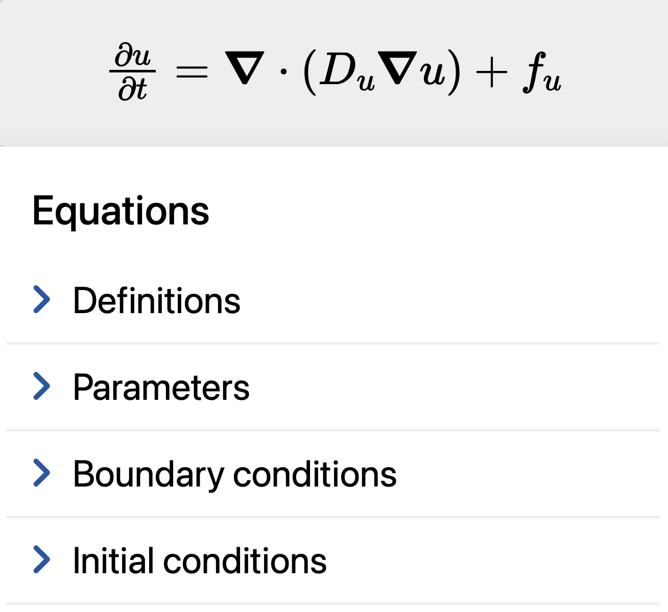
Here you can:
- See the equation being simulated, here $\pd{u}{t} = \vnabla\cdot(D_u\vnabla u) + f_u$.
- Set the named functions in the equations, here $D_u$ and $f_u$, under Definitions. These can be functions of any of the unknowns, space, and time (here $u$, $x$, $y$, and $t$), and of any parameters that will be defined further down the panel.
- Set the value of any extra parameters.
- Set the boundary conditions.
- Set the initial conditions.
- Set the number and type of equations to be solved.
Domain shape
The default domain for solving PDEs is a 2D rectangle, $\domain = [0,L_x]\times[0,L_y]$, which fits the size of your browser window or phone screen. Throughout VisualPDE, we use coordinates $x\in[0,L_x]$ and $y\in[0,L_y]$.
You can force the domain to be a square, $\domain = [0,L]\times[0,L]$, by toggling off → Domain → Fill screen
Boundary conditions
The following boundary conditions are available to allow you to set the value of the function, or the value of its derivative, along the boundary $\boundary$ of the domain $\domain$:
- Periodic
- Dirichlet (e.g. $u\onboundary = 0$)
- Neumann (e.g. $\pd{u}{n}\onboundary = 0$)
- Robin (e.g. $(u + \pd{u}{n})\onboundary = 0$)
You can swap between boundary conditions by choosing → Boundary conditions and selecting from the list for each variable.
Initial conditions
You can specify the values to which the unknowns ($u$, $v$, $w$) are initialised when resetting the simulation. These expressions can be functions of $x$, $y$, the special string ‘RAND’ that assigns a random number in [0,1] to each point in the domain, along with any user-defined parameters and the images $I_S$ and $I_T$ (see the advanced documentation for more details). You can also use $L$, $L_x$ and $L_y$.
Changing the equations
The simplest system VisualPDE can solve is a single PDE,
\[\pd{u}{t} = \vnabla \cdot (D_u \vnabla u) + f_u,\]where $D_u$ and $f_u$ are functions of $u$, $x$, $y$, and $t$ that you can specify.
The most complicated type is a coupled system of PDEs in four unknowns, $u$, $v$, $w$ and $q$:
\[\begin{aligned} t_u\pd{u}{t} &= \vnabla \cdot(D_{uu}\vnabla u+D_{uv}\vnabla v+D_{uw}\vnabla w+D_{uq}\vnabla q) + f_u,\\ \text{one of}\left\{\begin{matrix}\displaystyle t_v\pd{v}{t} \\ v\end{matrix}\right. & \begin{aligned} &= \vnabla \cdot(D_{vu}\vnabla u+D_{vv}\vnabla v+D_{vw}\vnabla w+D_{vq}\vnabla q) + f_v \vphantom{\displaystyle t_v\pd{v}{t}}, \\ &= \vnabla \cdot(D_{vu}\vnabla u+D_{vw}\vnabla w+D_{vq}\vnabla q) + f_v, \end{aligned}\\ \text{one of}\left\{\begin{matrix}\displaystyle t_w\pd{w}{t} \\ w\end{matrix}\right. & \begin{aligned} &= \vnabla \cdot(D_{wu}\vnabla u+D_{wv}\vnabla v+D_{ww}\vnabla w+D_{wq}\vnabla q) + f_w \vphantom{\displaystyle t_w\pd{w}{t}}, \\ &= \vnabla \cdot(D_{wu}\vnabla u+D_{wv}\vnabla v+D_{wq}\vnabla q) + f_w, \end{aligned}\\ \text{one of}\left\{\begin{matrix}\displaystyle t_q\pd{q}{t} \\ q\end{matrix}\right. & \begin{aligned} &= \vnabla \cdot(D_{qu}\vnabla u+D_{qv}\vnabla v+D_{qw}\vnabla w+D_{qq}\vnabla q) + f_q \vphantom{\displaystyle t_q\pd{q}{t}}, \\ &= \vnabla \cdot(D_{qu}\vnabla u+D_{qv}\vnabla v+D_{qw}\vnabla w) + f_q, \end{aligned} \end{aligned}\]where $D_{uu}, \dots, D_{qq}$, $f_u, \dots, f_q$ and $t_u, \dots, t_q$ are functions of $u$, $v$, $w$, $q$, $x$, $y$ and $t$ that you can specify.
- You can change the number of unknowns by choosing → Advanced options → Num. species
- In systems of multiple unknowns, you can include terms representing cross-diffusion (e.g. $D_{uv}$, $D_{vu}$) by toggling → Advanced options → Cross diffusion
- In systems of multiple unknowns, you can choose between a differential or algebraic equation for some of the species (e.g. ‘$\partial w/\partial t=$’ or ‘$w=$’) by toggling → Advanced options → Algebraic w (or v or q)
More VisualPDE
For a comprehensive list of all the options that you can set in VisualPDE, check out the Advanced documentation, or discover what VisualPDE can solve in our brief summary.